![]() (3-4)
(3-4)
CHAPTER 3 - MEASUREMENT ACCURACY
5. Examples of Calibration Approaches and Accuracy Calculations
The following examples show different approaches to calibration and demonstrate other simple calculations and analyses that can be done concerning accuracy. These calculations can be used to investigate how well a water provider or user is measuring flow. Also, some of the example analyses will help select secondary head measuring equipment and will help determine when maintenance or replacement is needed.
(a) Number of Significant Figures in Computations
Although accuracy is necessary in computing discharges from data gathered in the field, the computations should not be carried out to a greater number of significant figures than the quality of the data justifies. Doing so would imply an accuracy which does not exist and may give misleading results. For example, suppose it is desired to compute the discharge over a standard contracted rectangular weir using the formula:
![]() (3-4)
(3-4)
where:
Q = the discharge in ft3/s
C = 3.33, a constant for the weir
L = the length of the weir in feet (ft)
h1 = the observed head on the weir (ft)
If the length of the weir is 1.50 ft and the observed head is 0.41 ft, the significant equation output is 1.24 ft3/s.
As a rule, in any computation involving multiplication or division in which one or more of the numbers is the result of observation, the answer should contain the same number of significant figures as is contained in the observed quantity having the fewest significant figures. In applying this rule, it should be understood that the last significant figure in the answer is not necessarily correct, but represents merely the most probable value.
(b) Calibration of an Orifice
The calibration of a submerged rectangular orifice requires measuring head for a series of discharges, covering the full range of operation, with another more precise and accurate system sometimes called a standard control. Based on hydraulic principles, discharge varies as the square root of the head differential, and the equation for discharge through a submerged orifice can be written as:
![]() (3-5)
(3-5)
where:
Q = discharge
g = acceleration caused by gravity
![]() h = upstream head minus
the head on the downstream side of the orifice
h = upstream head minus
the head on the downstream side of the orifice
A = the area of the orifice
Cd = coefficient of discharge
Also, the coefficient of discharge, Cd, must be determined experimentally for any combination of orifice shape, measuring head locations, and the location of orifice relative to the flow boundaries. The coefficient has been found to be constant if the orifice perimeter is located away from the approach channel boundary at least a distance equal to twice the minimum orifice opening dimensions. Values of the discharge coefficient calculated by putting the measured calibration data into equation 3-5 may be constant within experimental error if the orifice geometry complies with all the requirements for standard orifices throughout the calibration range.
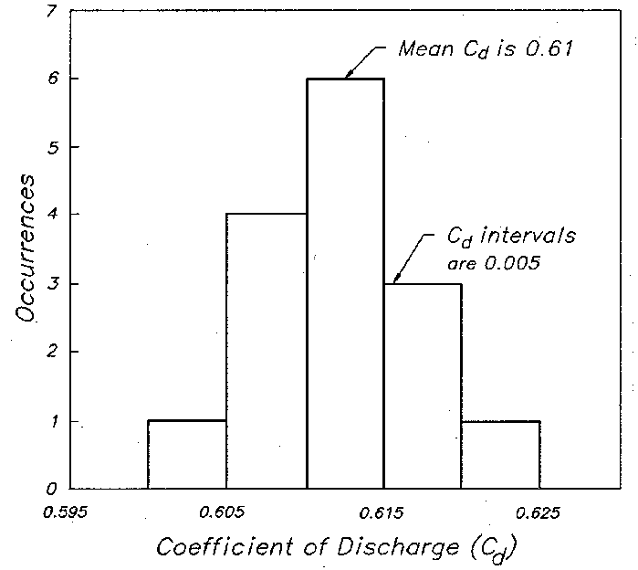
An example set of discharge data is shown in table 3-1. The theoretical hydraulic equation 3-5 was used to compute values of the coefficient of discharge, Cd. The mean of the values (0.61) is the most probable equation coefficient based on 15 readings. The deviation or spread of individual coefficient values from the mean value would be the measure of the uncertainty of the measuring system as used during the calibration. The deviation of coefficient values is an indication of how well the calibration was done. Therefore, accuracy statements should also include statements concerning the head reading technique capability and the accuracy of the standard device used to measure discharge. If several orifices of the same size were calibrated together, then the accuracy statements can be made concerning limits of fabrication and installation of the orifices.
The histogram of the same data as shown on figure 3-1 was developed by splitting the range of discharge values into five 0.005-ft3/s intervals. Then the data were tallied as they occurred in each interval. The plotted values of occurrence approach a symmetrical bell shape curve centered around the mean of 0.61, indicating that the data are random or normally distributed and that enough data were obtained to determine a meaningful average value for the discharge coefficient.
|
|
||
|
|
|
|
|
3.702 |
0.253 |
0.611 |
|
3.613 |
0.245 |
0.606 |
|
3.545 |
0.232 |
0.608 |
|
3.361 |
0.209 |
0.611 |
|
3.267 |
0.197 |
0.616 |
|
3.172 |
0.189 |
0.606 |
|
3.005 |
0.163 |
0.618 |
|
2.924 |
0.161 |
0.605 |
|
2.842 |
0.154 |
0.602 |
|
2.565 |
0.127 |
0.598 |
|
2.450 |
0.109 |
0.616 |
|
2.323 |
0.100 |
0.610 |
|
1.986 |
0.073 |
0.611 |
|
1.813 |
0.060 |
0.615 |
|
1.640 |
0.050 |
0.609 |
| Standard deviation = | E Cd = 9.142 Cd Avg = 0.610 S = 0.006 |
|
|
|
The measure of the spread of repeated measurements such as the discharge coefficient is the estimated standard deviation, which when using the form of equation 3-1 is written as:
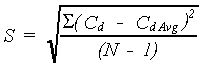 (3-6)
(3-6)
where ![]() denotes summation, and
N is the number of Cd values. The value of S
is the estimate of standard deviation,
denotes summation, and
N is the number of Cd values. The value of S
is the estimate of standard deviation, ![]() ,
which is approached more closely as the number of samples, N,
becomes
larger. Formal, small sample statistical methods can be used to
evaluate
confidence bounds around S based on sample size. After N
has become large enough and normal distribution is verified, all
previous
and subsequent data are expected to fall within the bounds of +S,
+2S, and +3S for about 68.3, 95.4, and
99.7
percent confidence levels, respectively.
,
which is approached more closely as the number of samples, N,
becomes
larger. Formal, small sample statistical methods can be used to
evaluate
confidence bounds around S based on sample size. After N
has become large enough and normal distribution is verified, all
previous
and subsequent data are expected to fall within the bounds of +S,
+2S, and +3S for about 68.3, 95.4, and
99.7
percent confidence levels, respectively.
(c) Error Analysis of Calibration Equation
Often, structural compromise, in Parshall flumes for example, is such that hydraulic theory and analysis cannot determine the exponents or the coefficients. These devices must be calibrated by measuring head for a series of discharges well distributed over the flow range and measured with another, more accurate device. The data can be plotted as a best fit curve on graph paper. However, determination of equations for table generation would be preferable.
Parshall flumes and many other water measuring devices have close approximating equations of the form:
![]() (3-7)
(3-7)
If the data plot as a straight line on log-log graph paper, then equation 3-7 can be used as the calibration form, and a more rigorous statistical approach to calibration is possible. This equation can be linearized for regression analysis by taking the log of both sides, resulting in:
![]() (3-8)
(3-8)
Although a regression analysis can produce correlation coefficients greater than 0.99, with 1.0 being perfect, large deviations in discharge can exist. These deviations include error of estimating head between scale divisions for both the test and comparison standard devices, known errors of the comparison standard, and possible offset from linearity of the measuring device. For example, a laboratory calibration check of a 9-inch Parshall flume in a poor approach situation, using a venturi meter as the comparison standard, resulted in a correlation coefficient of 0.99924, an equation coefficient, C, of 3.041, and an exponent of 1.561 using 15 values of discharge versus measuring head pairs. For the properly set flume in tranquil flow, C is 3.07 and n is 1.56.
To overcome the defect of using correlation coefficients that are
based
on log units, the flume measuring capability should be investigated in
terms of percent discharge deviations, ![]() Q,
or expressed as:
Q,
or expressed as:
 (3-9)
(3-9)
where:
![]() Q% = percent deviation
of discharge
Q% = percent deviation
of discharge
QCs = measured comparison standard discharge
QEq = discharge computed using measured heads and the regression equation
Then, calculate the estimate of standard deviation, S, and
substitute
![]() Q% for Cd
in equation 3-6 from the previous example. For the Parshall flume
example,
S was about 3.0 percent. The maximum deviation for the example
flume
was about -10 percent, and the average deviation was about 0.08 percent
discharge, which is a small bias from the expected zero. Because of
this
small bias combined with a maximum absolute deviation of about 3S,
the error was considered normally distributed, and the sample size, N,
was considered adequate. Examples will be used to describe the next
four
sections.
Q% for Cd
in equation 3-6 from the previous example. For the Parshall flume
example,
S was about 3.0 percent. The maximum deviation for the example
flume
was about -10 percent, and the average deviation was about 0.08 percent
discharge, which is a small bias from the expected zero. Because of
this
small bias combined with a maximum absolute deviation of about 3S,
the error was considered normally distributed, and the sample size, N,
was considered adequate. Examples will be used to describe the next
four
sections.
(d) Error Analysis of Head Measurement
A water project was able to maintain a constant discharge long enough to obtain ten readings of head, h1. These readings are listed in the first column of table 3-2.
This example process provides information on repetitions of hook gage readings but does not tell the whole story about system accuracy. Good repeatability combined with poor accuracy can be likened to shooting a tight, low scoring group on the outer margin of a target. Repetition is a necessary aspect of accuracy but is not sufficient by itself.
|
|
||
|
|
|
|
|
1.012 |
-0.0011 |
0.00000121 |
|
1.017 |
0.0039 |
0.00001521 |
|
1.014 |
0.0009 |
0.00000081 |
|
1.010 |
-0.0031 |
0.00000961 |
|
1.015 |
0.0019 |
0.00000361 |
|
1.013 |
-0.0001 |
0.00000001 |
|
1.012 |
-0.0011 |
0.00000121 |
|
1.014 |
0.0009 |
0.00000081 |
|
1.013 |
-0.0001 |
0.00000001 |
|
1.011 |
-0.0021 |
0.00000441 |
| h1Avg = 1.013 | S = (0.00003690)0.5 = 0.0061 | |
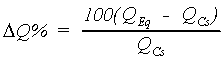
(e) Determining the Effect of Head Measurement on Accuracy
Say a water provider or user measures a discharge of 8.96 ft3/s using a 3-ft suppressed weir with a staff gage estimating readings to +0.01 ft. The head reading was 0.93 ft, and the water provider or user wants to investigate how much this estimate of head affects the accuracy of the discharge measurement. Assume that the reading and discharge are actual values and then add and subtract 0.01 ft to and from the 0.93-ft head reading, which gives heads of 0.94 ft and 0.92 ft. Discharges by table or equation for these new heads are 9.10 ft3/s and 8.82 ft3/s. The difference of these discharges from 8.96 ft3/s in both cases is 0.14 ft3/s, but of a different sign in each case. Thus, an uncertainty in discharge of +0.14 ft3/s was caused by an uncertainty of +0.01 ft in head reading. The uncertainty of the discharge measurement caused by estimating between divisions on the staff gage expressed in percent of actual discharge is calculated as follows:
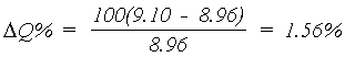
and:
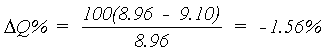
This calculation shows that estimating the staff gage +0.01 ft contributes up to +1.6 percent error in discharge at flows of about 9 ft3/s. Both calculations are required because both could have been different depending on the discharge equation form and the value of discharge relative to measuring range limits.
(f) Computation to Help Select Head Measuring Device
An organization uses several 3-ft weirs and wants to decide between depending on staff gage readings or vernier hook gage readings in a stilling well. From experience, they think that the staff gage measures head to within +0.01 ft, and the hook gage measures to within +0.002 ft. The equation for the 3-ft weir in the previous example calculation is:
![]() (3-10)
(3-10)
Using this equation and making calculations similar to the previous example, they produce table 3-3.
It is assumed that the water provider does not want to introduce more than 2 percent error caused by precision of head measurement. This amount of error is demarcated by the stepped line through the body of table 3-3. If the water providers needed to measure flow below 7 ft3/s, they would have to use stilling wells and vernier point gages. This line shows that heads could be measured with a staff gage at locations where all deliveries exceed about 7 ft3/s. They could select a higher cut-off percentage based on expected frequency of measurements at different discharges. The results of this type of analysis should be compared to the potential accuracy of the primary part of the measuring system.
|
|
|||
|
Discharge (ft3/s) |
Equation Head (ft) |
Percent deviation of discharge at calibration head at a plus
|
|
|
|
|
||
|
Deviation (%) |
Deviation (%) |
||
|
18 |
1.481 |
0.25 |
1.0 |
|
9 |
0.933 |
0.37 |
1.6 |
|
5 |
0.630 |
0.53 |
2.7 |
|
3 |
0.448 |
0.72 |
3.6 |
|
2 |
0.342 |
0.92 |
4.4 |
|
1 |
0.216 |
1.40 |
7.0 |
(g) Relationship Between Full Scale and Actual
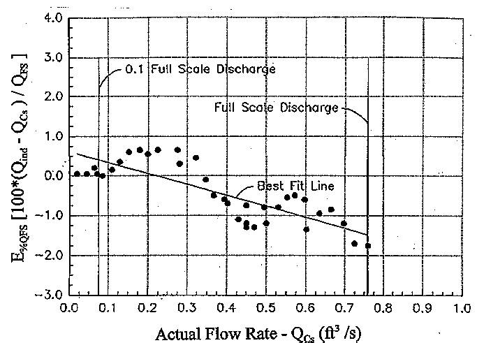
Before buying several small acoustic flowmeters, a water provider requested that one be tested to see if the manufacturer's claim of accuracy was really true. Because the acoustic flowmeter is an electronic device, the manufacturer prefers to express calibration performance in terms of full-scale accuracy. The manufacturer claimed +2 percent full-scale accuracy. Full-scale percentage accuracy is defined as the difference between comparison standard measured discharge and output flowmeter discharge relative to full-scale discharge. Full-scale discharge is equivalent to the discharge upper range limit of the flowmeter. The error in percent full-scale discharge is calculated using equation 3-3.
Figure 3-2 shows the test data for the acoustic flowmeter that was checked. Full-scale discharge is 0.768 ft3/s as shown by the vertical line on the right. The standard comparison discharge was measured using a volumetric calibration tank and electronic timer which can measure discharge within 0.5 percent. This plot indicates the
|
|
fit line slopes down to the right and passes through the zero error company claim of +2.0-percent full-scale accuracy is true. The best axis to the left of midrange. This meter could be made to have a better full-scale accuracy by shifting the meter output vertically and/or tilting its output by electronics or computer programming.
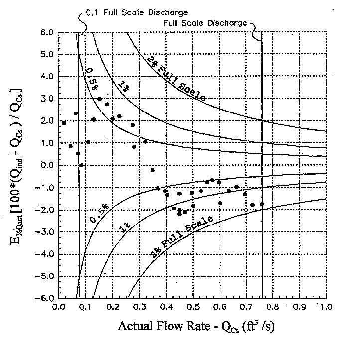
The same data were converted and plotted in terms of percent comparison standard error of discharge using equation 3-11 on figure 3-3. To compare error in percent of actual discharge, E%Qact, with error in percent full-scale discharge, E%QFS, calculated contours of equal percent full scale were also plotted on figure 3-3.
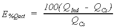 (3-11)
|
|
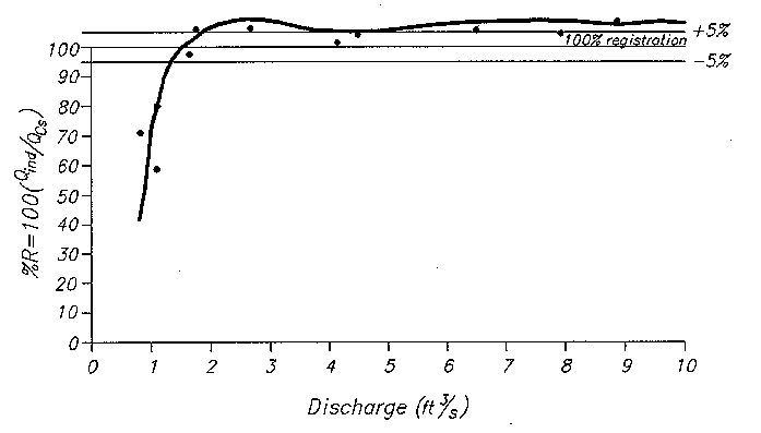
(h) Percent Registration Calibration
Another way accuracy and calibration are expressed is in terms of percent registration. Calibration checks for open flow propeller meters are often presented this way. Percent registration is defined as:
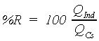 (3-12)
A typical calibration check of a propeller meter mounted at the end of a pipe is plotted on figure 34. For this flowmeter, percent registration drops steeply below a discharge of 1 ft3/s. This result clearly indicates some of the problems of measuring near the lower range limits of this flowmeter. A slight increase of bearing friction will shift the dropping part of the curve to the right because the discharge at which the propeller will not turn will increase. Thus, in effect, the range is shortened on its low discharge end. The percent registration on the flat part of the curve near maximum registration will also decrease with age and wear of the flowmeter. In fact, the manufacturer may set meters, when they are new, to register high in anticipation of future wear. For example, they may set meters to read 3 to 5 percent high, expecting wear to lower the curve to about 100 percent registration at about mid-life of the flowmeter.
|
|